Adversarial Attacks
Introduction
The goal of an adversial attack is to specifically add “noise” (or some other carefully picked input) to an image in such a manner that the human reader does not notice anything different, but a well-trained machine model will end up classifying the image incorrectly. For example, we have an image of a cat, but with some pixel changes here and there, we wish for the model to identify our cat as something else; perhaps a dog or even a car.
The most well known example (which comes from the original paper) is as follows
 Clearly we can tell that the image is of a panda. This noise in the middle is scaled using “ε” and then added to the image on the left to produce our right image which still looks like a panda but our model is 99.3% confident that we now have a gibbon instead. Crazy right?!?
Today we will be taking a closer look at white-box attacks. A white box attacks allows for the adversary to know the specifics of the model archetitecture, parameters, gradients, etc which allow for easier targeting. White-box attacks often exploit the model’s output gradient to generate fake examples which aim to look real.
Algorithm 1 — FGSM
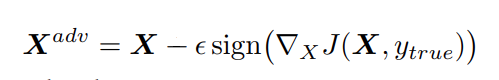
FGSM stand for Fast Gradient Sign Method. First introduced as a concept in this 2014 paper, its purpose was to provide a simple way to make adversarial examples of nonlinear models. The reason it is labelled as fast is that this method only requires one step which can be made efficient through backpropagation. It works by simply maximizing the loss function then adding it back to the original image with respect to the sign of the gradient to produce our adversarial image.
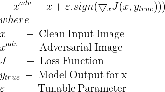 This is the mathematical formulation. The reason FGSM works is that we are slowly shifting the image so that the loss towards the correct label grows so much so that our model will relabel our image something else. In the example above, we are moving away from the true panda class and shifting instead to some other incorrect one. The algorithm does not care what the other one is as long as it is not panda.
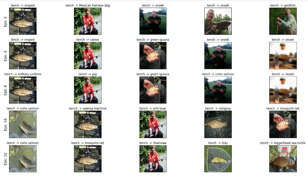
Here are some examples of misclassifications attacking a pretrained resnet50 model using images from the ImageNette dataset. ImageNette is a much smaller subset of ImageNet which is a common training set for many neural networks. For purposes of our study, ImageNette works as it is significantly smaller than ImageNet and allows for considerably speedier runtimes.
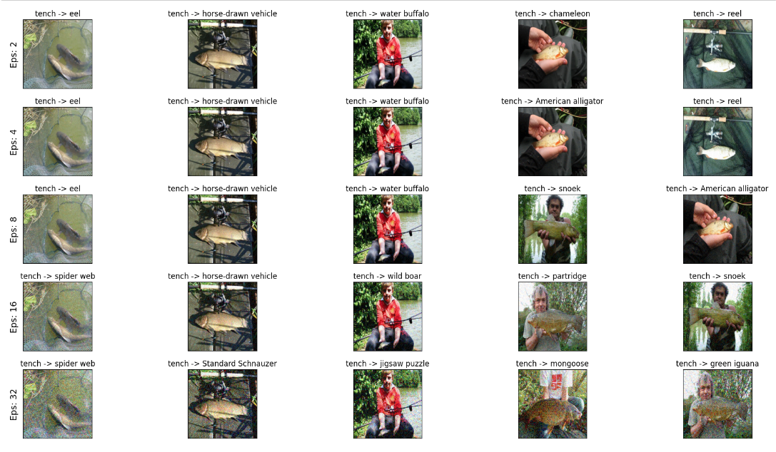
I might clarify that tench is a type of aquatic fish also known as doctor fish. We see that for some values, the misclassifications are rather reasonable. Eel and snoek are both types of fish and reel (fishing reel) is identified for another image with both the tench and the rod. However, with an increase in epsilon, the results stray away from aquatic animals and give results such as wild boar and partridge.
Algorithm 2 — i-FGSM
i-FGSM, iterative FGSM or also known as Basic Iterative Method (BIM), is an extension of FGSM as its title would suggest. The method is iterative as it performs FGSM multiple times
This is the equation used as mentioned in the 2017 paper
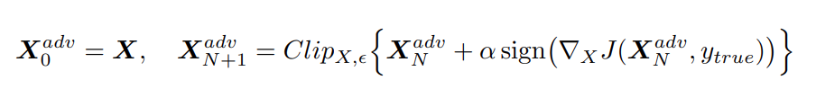
The number of iterations that we perform is not static. Instead we apply a heuristic min(ε + 4, 1.25ε) as the 2017 paper suggests. The point of using this heuristic is to limit the computational costs while still aimiming to reach the best possible results. Due to this being an iterative method, we must compute a step of gradient descent for every iteration which is why this method is much slower to run than FGSM. There are clear benefits however as will be reviewed in depth later down in the post. But from a cursory glance, an iterative method will allow for the error to stray further and further away from the input as we move the error function in the direction of the gradient.
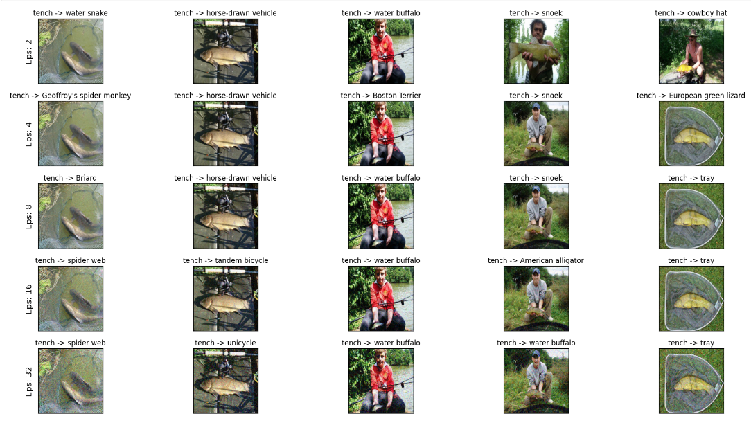
Similarly, here are some misclassified images from ImageNette
Algorithm 3 — L.L.Class
LLC, least-likely class, is introduced in the 2017 as iterative least-likely class method with equation
As the name would suggest, the goal of this method is to shift our original image towards an unlikely target class. The idea behind this method is to allow for classifications of “meaningful interest” as for larger models trained on larger datasets with more specific labels, we do not really want one type of cat to be misclassified as another breed of cat. The aim is to allow for more classifications that are clearly outrageous and “interesting”. The equation
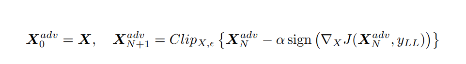
Here I’ll be using a simplified approach from the one introduced in the paper which consists only of one iteration
 (Running on GCP vm is expensive so I’ll take this shortcut approach but for individuals interested in better quality outputs, iterative method is better just much slower to run)
Similarly, here are some misclassified images from ImageNette
Conclusions to Drawn
Here is a graph showing the accuracies of our model on the perturbed images.
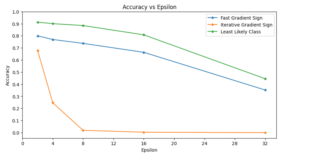
Obviously increasing the epsilon values helps to create images that are “more wrong”. But as epsilon increases too much, the images become noticeably more granular and less like the original. Too many pixels changed and shifted is not ideal as the goal is to still provide an image that looks much like the original one. Looking at the graph, we will notice that the iterative method is much better performancewise. This is due to the fact that the interative method allows for much finer exploitations and do not destroy our original image as much even at higher epsilon values.
Summarizing some ideas from the two papers linked above, it is clear that there are still ways to improve upon modern neural networks. “The existence of adversarial examples suggests that being able to explain the training data or even being able to correctly label the test data does not imply that our models truly understand the tasks we have asked them to perform.” 2014 The prevalently used gradient-based optimization methods allows for confident fitting of training set examples but leaves much room for our rather simple and linear algorithms to find holes and random pixels to exploit.
Some Final Thoughts
Proper design for protection against strong adversarial attacks is an important area that remains unsolved as of the present. The simplicity of these adversarial algorithms and their effectiveness against models which are trained for weeks on end being fed trillions of bytes of data shows that there is still much work left to be done. The simple truth is that models function differently than how we may have initially designed them to operate. Small pertubations of even single pixels can arbitrarily fool complex models. Of recent, twists on implementations of GAN have been tried as possible defense mechanisms. However, GAN’s themselves are very costly computationally to both train and run. Incorrect/Incomplete training can lead to poor results. The parameters that a GAN model may learn can also vary between runs and makes results hard to replicate. I’ll being showing some basic ideas of such concepts in another blogpost. Be on the lookout!